Google Sheets is a great tool to work with your data. You can store it, clean it, organize it, manipulate it, analyze it, scrape webpages with it and download it in several formats.

This tutorial will give you a basic overview of the text formulas Google Sheets offers you, also with some basic, most used functions for strings.

It will assume that you already knows how to do the most basic things, like removing or adding columns and rows (just right click them) and sheet tabs, for instance. We won’t talk about formatting the data here, with colors and fonts.

For this, you will need:

1. Access the exemple data
2. A Google account
3. Going to Google Spreadsheets page

---

Getting started

Access the example data in the link above about newsrooms based in New York city - with addresses, social media following numbers, description and even latitude and longitude.

Make a copy of this file by doing File -> Make a Copy.

After that, you will see we created a new sheet tab on the bottom, called “Test here”. This was made so you have a secure environment to work with your data without erasing the original dataset and having the trouble to look for the original file to copy again.

Always make a copy of the original dataset

You can either copy and paste the data in the second sheet or duplicate the original file as another sheet.

Putting values together

Sometimes, you might need to put together values within certain cells, for whatever reason you deem necessary. For, there are two basic formulas - CONCAT for two values, and CONCATENATE for more than two values. The application is the same.

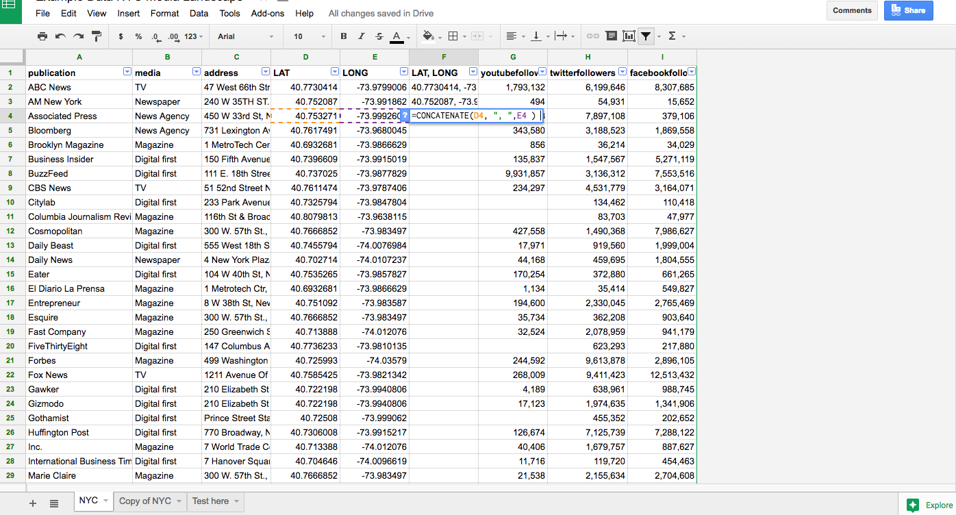
In our example dataset, take a look at the LAT and LONG columns. Some people like to have that info in the same column. Lets do it then.

Create a new column on the side of the LONG column and apply the formula:

=CONCATENATE(D1, ", ",E1 )

We are using CONCATENATE because we will want to separate the values with a comma - making it three strings to put together. If you for some reason don’t want the comma, you may use CONCAT.

After that, just apply the same formula to the other cells, by dragging the blue square in the corner of the cell.

You can also use the JOIN formula, which is very similar, but allows you to use a specified delimiter.

Splitting values

As with merging cells, is also very common that you will need to split values within a cell. There is a basic command for that, the SPLIT function.

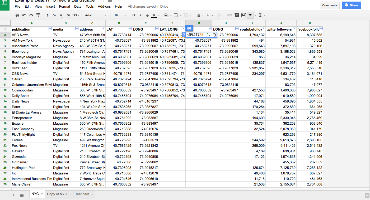
You have to determine with character will be used to tell your cell to split into. Lets say you now want to undo the CONCAT operation you did, and now need to separate LAT and LONG.

First, you are splitting two values, so you will need two more columns. Create them and apply the formula:

=SPLIT(F1, ", ")

This way, your telling the formula to split that values on that cell based on the comma your have there. The split value will disappear.

Find and replace

Finding and replacing values may be one of the most useful tools to clear and manipulate your data. And it might, just as well, be one of the most dangerous one. Be sure to use it carefully.

As you can see in our dataset, the social media following count numbers are separated by commas. That is nice to make the number clearer, but if may cause confusion when using CSV or trying to parse data in charting tools. Lets clear those commas and make it a “clean” number.

Make sure you select ONLY the columns your are trying to change. They will be highlighted in blue like in the picture below. To do that, hold SHIFT and click on the column top headers (the letters).

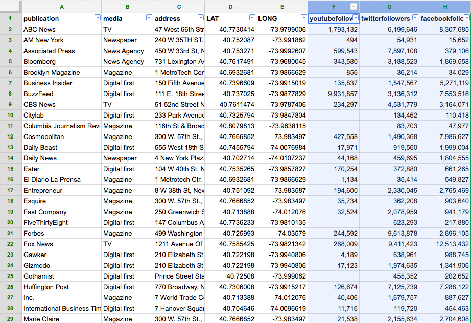
WARNING: If you fail or forget to do that, you may put all your dataset at risk, in some cases even other sheet tabs, as you might erase all the commas in that entire dataset, even the ones you don’t want to.

Then proceed to Edit -> Find and Replace.

The Find is where you will insert the character you want to change or remove, in this case the comma. The Replace with is where you put the value you want to add. Since are cleaning the number not to have any separator, we will leave it blank (no spaces). You can add a few parameters, like selecting specific ranges in your dataset to modify - but in this canse we want the entire column.

Click the Replace all button.

If nothing happens, it is because your spreadsheet formatting settings are adding the commas automatically, as it recognizes the values as numbers.

There are some ways around this issue.

1. Go to Format -> Number -> Plain Text - this will tell your cell to recognize the cell as a string, not a number. Do the Find and Replace process again now. This can be a faster approach.
2. Format -> Number -> More Formats -> Custom Number Formats, and select a number format without commas or numbers. This could tell your whole spreadsheet to read numbers like that, if you want. This can be a better practices approach.

TIP: Another approach for this is to use the SUBSTITUTE function. This is safer and more accurate, but certainly more intricate.

This this function to solve the same problem:

=SUBSTITUTE(H2, ",", "")

This tells that in the cell H2, we are substituting comma for nothing. If you want to just substitute the

---

Be a pro

Check out this list of functions and try them out.

The TRIM function is pretty useful when you want to extract certain parts of a text in a cell or cut white spaces.

---